第 2 章 使用 R 函数
2.1 金融时间序列对象与 base 包中的函数
所需的 R 包
下面介绍几个与金融时间序列分析关系紧密的 R 函数,这些函数的分析对象即可以是多元时间序列也可以是单边量时间序列。
set.seed(1953)
data <-matrix(runif(18), ncol = 3)
charvec <-rev(paste("2009-0", 1:6, "-01", sep = ""))
charvec
## [1] "2009-06-01" "2009-05-01" "2009-04-01"
## [4] "2009-03-01" "2009-02-01" "2009-01-01"zoo:
xts:
timeSeries:
zoo:
xts:
timeSeries:
2.1.1 可以对金融时间序列对象应用 apply 函数吗?如何应用?
zoo:
##    Z.1    Z.2    Z.3
## 0.4165 0.5882 0.5857
xts:
##    X.1    X.2    X.3
## 0.4165 0.5882 0.5857
timeSeries:
##    S.1    S.2    S.3
## 0.4165 0.5882 0.5857
2.1.2 可以对金融时间序列对象应用 attach 函数吗?
应用 attach 函数之后,R 的数据库被纳入到工作区,如此一来,只需在 R 中键入数据集的名称,便可调用该数据集。attach函数的对象只能是lists,data frames和environments。因此,attach 函数针对金融时间序列对象不可用。
zoo:
xts:
timeSeries:
## [1] "S.1" "S.2" "S.3"## GMT
## S.1 S.2 S.3
## 2009-06-01 0.5087 0.5740 0.9311
## 2009-05-01 0.4770 0.5737 0.3990
## 2009-04-01 0.1829 0.5913 0.8642
## 2009-03-01 0.4473 0.9652 0.6136
## 2009-02-01 0.6603 0.5932 0.4981
## 2009-01-01 0.2228 0.2319 0.20832.1.3 能对金融时间序列对象应用 diff 函数么?
base 包中,diff 函数的作用是返回对象的差分序列。该函数可用于金融时间序列分析对象。
zoo:
##                 Z.1        Z.2     Z.3
## 2009-02-01  0.43745  0.3612280  0.2898
## 2009-03-01 -0.21299  0.3720793  0.1155
## 2009-04-01 -0.26439 -0.3739671  0.2506
## 2009-05-01  0.29411 -0.0176171 -0.4652
## 2009-06-01 0.03172 0.0003665 0.5321## 2009-02-01 2009-03-01 2009-04-01 2009-05-01
## 0.43745 -0.21299 -0.26439 0.29411
## 2009-06-01
## 0.03172xts:
##                 X.1        X.2     X.3
## 2009-01-01       NA         NA      NA
## 2009-02-01  0.43745  0.3612280  0.2898
## 2009-03-01 -0.21299  0.3720793  0.1155
## 2009-04-01 -0.26439 -0.3739671  0.2506
## 2009-05-01  0.29411 -0.0176171 -0.4652
## 2009-06-01 0.03172 0.0003665 0.5321## X.1
## 2009-01-01 NA
## 2009-02-01 0.43745
## 2009-03-01 -0.21299
## 2009-04-01 -0.26439
## 2009-05-01 0.29411
## 2009-06-01 0.03172timeSeries:
## GMT
##                 S.1        S.2     S.3
## 2009-06-01       NA         NA      NA
## 2009-05-01 -0.03172 -0.0003665 -0.5321
## 2009-04-01 -0.29411  0.0176171  0.4652
## 2009-03-01  0.26439  0.3739671 -0.2506
## 2009-02-01  0.21299 -0.3720793 -0.1155
## 2009-01-01 -0.43745 -0.3612280 -0.2898## GMT
## S.1
## 2009-06-01 NA
## 2009-05-01 -0.03172
## 2009-04-01 -0.29411
## 2009-03-01 0.26439
## 2009-02-01 0.21299
## 2009-01-01 -0.437452.1.4 能对金融时间序列对象应用 dim 函数么?
dim 函数用于返回对象的维度。该函数适用于金融时间序列对象。
zoo:
## [1] 6 3## NULLxts:
## [1] 6 3## [1] 6 1timeSeries:
## [1] 6 3## [1] 6 12.1.5 能对金融时间序列对象应用 rank 函数吗?rank函数返回对象中每个元素的顺序位置。仅适用于 timeSeries类型的金融时间序列对象。
zoo
xts:
timeSeries:
## GMT
##            S.1 S.2 S.3
## 2009-06-01   5   3   6
## 2009-05-01   4   2   2
## 2009-04-01   1   4   5
## 2009-03-01   3   6   4
## 2009-02-01   6   5   3
## 2009-01-01 2 1 1## GMT
## S.1
## 2009-06-01 5
## 2009-05-01 4
## 2009-04-01 1
## 2009-03-01 3
## 2009-02-01 6
## 2009-01-01 22.1.6 能对金融时间序列对象应用 rev 函数么?
rev 函数用于返回对象的逆排列。
zoo:
##               Z.1    Z.2    Z.3
## 2009-01-01 0.5087 0.5740 0.9311
## 2009-02-01 0.4770 0.5737 0.3990
## 2009-03-01 0.1829 0.5913 0.8642
## 2009-04-01 0.4473 0.9652 0.6136
## 2009-05-01 0.6603 0.5932 0.4981
## 2009-06-01 0.2228 0.2319 0.2083## 2009-01-01 2009-02-01 2009-03-01 2009-04-01
## 0.5087 0.4770 0.1829 0.4473
## 2009-05-01 2009-06-01
## 0.6603 0.2228xts:
## X.1 X.2 X.3
## 2009-01-01 0.5087 0.5740 0.9311
## 2009-02-01 0.4770 0.5737 0.3990
## 2009-03-01 0.1829 0.5913 0.8642
## 2009-04-01 0.4473 0.9652 0.6136
## 2009-05-01 0.6603 0.5932 0.4981
## 2009-06-01 0.2228 0.2319 0.2083## X.1
## 2009-01-01 0.5087
## 2009-02-01 0.4770
## 2009-03-01 0.1829
## 2009-04-01 0.4473
## 2009-05-01 0.6603
## 2009-06-01 0.2228timeSeries:
## GMT
## S.1 S.2 S.3
## 2009-01-01 0.2228 0.2319 0.2083
## 2009-02-01 0.6603 0.5932 0.4981
## 2009-03-01 0.4473 0.9652 0.6136
## 2009-04-01 0.1829 0.5913 0.8642
## 2009-05-01 0.4770 0.5737 0.3990
## 2009-06-01 0.5087 0.5740 0.9311## GMT
## S.1
## 2009-01-01 0.2228
## 2009-02-01 0.6603
## 2009-03-01 0.4473
## 2009-04-01 0.1829
## 2009-05-01 0.4770
## 2009-06-01 0.50872.1.7 能对金融时间序列对象应用 sample 函数吗?
sample 函数用于从一组数据中进行返回或者不返回抽样。
zoo:
## 2009-01-01 2009-02-01 2009-03-01 2009-04-01
## 0.2228 0.6603 0.4473 0.1829
## 2009-05-01 2009-06-01
## 0.4770 0.5087xts:
## X.1
## 2009-01-01 0.2228
## 2009-02-01 0.6603
## 2009-03-01 0.4473
## 2009-04-01 0.1829
## 2009-05-01 0.4770
## 2009-06-01 0.5087timeSeries:
## GMT
## S.1 S.2 S.3
## 2009-05-01 0.4770 0.5737 0.3990
## 2009-04-01 0.1829 0.5913 0.8642
## 2009-03-01 0.4473 0.9652 0.6136
## 2009-06-01 0.5087 0.5740 0.9311
## 2009-01-01 0.2228 0.2319 0.2083
## 2009-02-01 0.6603 0.5932 0.4981## GMT
## S.1
## 2009-06-01 0.5087
## 2009-02-01 0.6603
## 2009-05-01 0.4770
## 2009-01-01 0.2228
## 2009-03-01 0.4473
## 2009-04-01 0.18292.1.8 能对金融时间序列对象应用 scale 函数吗?若能,其实如何操作的?
scale 函数的作用是将对象进行中心化/标准化。
zoo:
## Z.1 Z.2 Z.3
## 2009-01-01 -1.0674 -1.53452 -1.3644
## 2009-02-01 1.3434 0.02131 -0.3167
## 2009-03-01 0.1696 1.62387 0.1007
## 2009-04-01 -1.2874 0.01317 1.0068
## 2009-05-01 0.3335 -0.06270 -0.6750
## 2009-06-01 0.5083 -0.06112 1.2485
## attr(,"scaled:center")
## Z.1 Z.2 Z.3
## 0.4165 0.5882 0.5857
## attr(,"scaled:scale")
## Z.1 Z.2 Z.3
## 0.1815 0.2322 0.2766##
## 2009-01-01 -1.0674
## 2009-02-01 1.3434
## 2009-03-01 0.1696
## 2009-04-01 -1.2874
## 2009-05-01 0.3335
## 2009-06-01 0.5083
## attr(,"scaled:center")
## [1] 0.4165
## attr(,"scaled:scale")
## [1] 0.1815xts:
## X.1 X.2 X.3
## 2009-01-01 -1.0674 -1.53452 -1.3644
## 2009-02-01 1.3434 0.02131 -0.3167
## 2009-03-01 0.1696 1.62387 0.1007
## 2009-04-01 -1.2874 0.01317 1.0068
## 2009-05-01 0.3335 -0.06270 -0.6750
## 2009-06-01 0.5083 -0.06112 1.2485## X.1
## 2009-01-01 -1.0674
## 2009-02-01 1.3434
## 2009-03-01 0.1696
## 2009-04-01 -1.2874
## 2009-05-01 0.3335
## 2009-06-01 0.5083timeSeries:
## GMT
## S.1 S.2 S.3
## 2009-06-01 0.5083 -0.06112 1.2485
## 2009-05-01 0.3335 -0.06270 -0.6750
## 2009-04-01 -1.2874 0.01317 1.0068
## 2009-03-01 0.1696 1.62387 0.1007
## 2009-02-01 1.3434 0.02131 -0.3167
## 2009-01-01 -1.0674 -1.53452 -1.3644## GMT
## S.1
## 2009-06-01 0.5083
## 2009-05-01 0.3335
## 2009-04-01 -1.2874
## 2009-03-01 0.1696
## 2009-02-01 1.3434
## 2009-01-01 -1.06742.1.9 能对金融时间序列对象应用 sort 函数吗?
sort 函数的作用是是将对象进行自然顺序排列或者逆序排列。具体可以参考 order 函数。
zoo:
## 2009-01-01 2009-02-01 2009-03-01 2009-04-01
## 0.2228 0.6603 0.4473 0.1829
## 2009-05-01 2009-06-01
## 0.4770 0.5087xts:
## X.1
## 2009-01-01 0.2228
## 2009-02-01 0.6603
## 2009-03-01 0.4473
## 2009-04-01 0.1829
## 2009-05-01 0.4770
## 2009-06-01 0.5087timeSeries:
## GMT
## S.1 S.2 S.3
## 2009-01-01 0.2228 0.2319 0.2083
## 2009-02-01 0.6603 0.5932 0.4981
## 2009-03-01 0.4473 0.9652 0.6136
## 2009-04-01 0.1829 0.5913 0.8642
## 2009-05-01 0.4770 0.5737 0.3990
## 2009-06-01 0.5087 0.5740 0.9311## GMT
## S.1
## 2009-01-01 0.2228
## 2009-02-01 0.6603
## 2009-03-01 0.4473
## 2009-04-01 0.1829
## 2009-05-01 0.4770
## 2009-06-01 0.50872.1.10 能对金融时间序列对象应用 start 和 end 函数吗?
start函数和end函数用于返回对象的头部数据和尾部数据。针对金融时间序列对象时,其返回的是时间戳的头部部分和尾部部分。
zoo:
## [1] "2009-01-01"## [1] "2009-06-01"## [1] "2009-01-01"## [1] "2009-06-01"xts:
## [1] "2009-01-01"## [1] "2009-06-01"## [1] "2009-01-01"## [1] "2009-06-01"timeSeries:
## GMT
## [1] [2009-01-01]## GMT
## [1] [2009-06-01]## GMT
## [1] [2009-01-01]## GMT
## [1] [2009-06-01]2.2 金融时间序列对象与 stats 包中的函数
所需 R 包
下面从 stats 包中选取一些与金融时间序列分析相关的函数进行介绍。
常规数据
测试数据为多元金融时间序列和单变量金融时间序列对象。
set.seed(1953)
data <-matrix(runif(18), ncol = 3)
charvec <-paste("2009-0", 1:6, "-01", sep = "")
charvec## [1] "2009-01-01" "2009-02-01" "2009-03-01"
## [4] "2009-04-01" "2009-05-01" "2009-06-01"zoo:
## Z.1 Z.2 Z.3
## 2009-01-01 0.5087 0.5740 0.9311
## 2009-02-01 0.4770 0.5737 0.3990
## 2009-03-01 0.1829 0.5913 0.8642
## 2009-04-01 0.4473 0.9652 0.6136
## 2009-05-01 0.6603 0.5932 0.4981
## 2009-06-01 0.2228 0.2319 0.2083xts:
## X.1 X.2 X.3
## 2009-01-01 0.5087 0.5740 0.9311
## 2009-02-01 0.4770 0.5737 0.3990
## 2009-03-01 0.1829 0.5913 0.8642
## 2009-04-01 0.4473 0.9652 0.6136
## 2009-05-01 0.6603 0.5932 0.4981
## 2009-06-01 0.2228 0.2319 0.2083timeSeries:
## GMT
## S.1 S.2 S.3
## 2009-01-01 0.5087 0.5740 0.9311
## 2009-02-01 0.4770 0.5737 0.3990
## 2009-03-01 0.1829 0.5913 0.8642
## 2009-04-01 0.4473 0.9652 0.6136
## 2009-05-01 0.6603 0.5932 0.4981
## 2009-06-01 0.2228 0.2319 0.2083zoo:
## 2009-01-01 2009-02-01 2009-03-01 2009-04-01
##     0.5087     0.4770     0.1829     0.4473
## 2009-05-01 2009-06-01
##     0.6603     0.2228
xts:
## X.1
## 2009-01-01 0.5087
## 2009-02-01 0.4770
## 2009-03-01 0.1829
## 2009-04-01 0.4473
## 2009-05-01 0.6603
## 2009-06-01 0.2228timeSeries:
## GMT
## S.1
## 2009-01-01 0.5087
## 2009-02-01 0.4770
## 2009-03-01 0.1829
## 2009-04-01 0.4473
## 2009-05-01 0.6603
## 2009-06-01 0.22282.2.1 能对金融时间序列对象应用 arima 函数么?
arima 函数的作用是对单变量时间序列对象建立 arima 模型。
zoo:
##
## Call:
## arima(x = z)
##
## Coefficients:
## intercept
## 0.417
## s.e. 0.068
##
## sigma^2 estimated as 0.0274: log likelihood = 2.27, aic = -0.55xts:
##
## Call:
## arima(x = x)
##
## Coefficients:
## intercept
## 0.417
## s.e. 0.068
##
## sigma^2 estimated as 0.0274: log likelihood = 2.27, aic = -0.55timeSeries:
##
## Call:
## arima(x = s)
##
## Coefficients:
## intercept
## 0.417
## s.e. 0.068
##
## sigma^2 estimated as 0.0274: log likelihood = 2.27, aic = -0.552.2.2 能对金融时间序列对象应用 acf 函数吗?
acf 函数用以返回对象的自协方差和自相关序列。pacf函数用以返回对象的偏自相关序列。ccf 函数用以返回互相关序列和互协方差序列。
zoo:
xts:
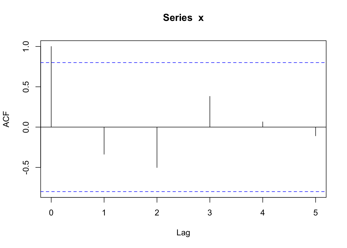
##
## Autocorrelations of series 'x', by lag
##
## 0 1 2 3 4 5
## 1.000 -0.337 -0.502 0.382 0.065 -0.109timeSeries:
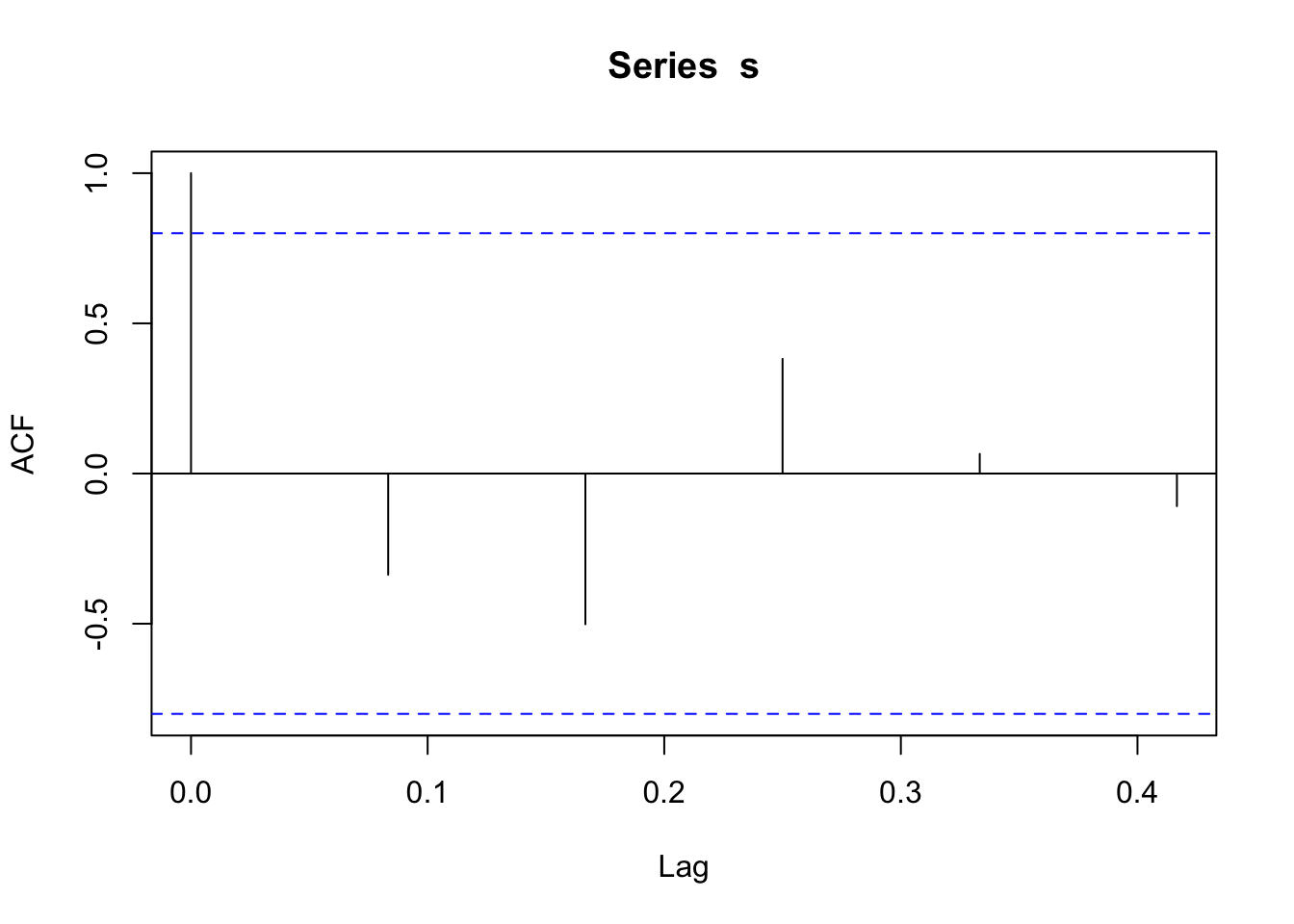
##
## Autocorrelations of series 's', by lag
##
## 0.0000 0.0833 0.1667 0.2500 0.3333 0.4167
## 1.000 -0.337 -0.502 0.382 0.065 -0.1092.2.3 能对金融时间序列对象应用 cov 函数吗?
var 函数、cov 函数和 cor 函数用以返回对象 x 的方差、协方差或者 x,y 的协相关系数。
如果 x,y 是矩阵形式,其返回结果为对象 x 的列于对象 y 的列的协方差或者协相关系数。应用于 zoo、xts 和 timeSeries 对象是表现如下:
zoo:
## [1] 0.03292## Z.1 Z.2 Z.3
## Z.1 0.032925 0.01578 0.001619
## Z.2 0.015783 0.05391 0.028640
## Z.3 0.001619 0.02864 0.076510## Z.1 Z.2 Z.3
## Z.1 0.032925 0.01578 0.001619
## Z.2 0.015783 0.05391 0.028640
## Z.3 0.001619 0.02864 0.076510## Z.1 Z.2 Z.3
## Z.1 1.00000 0.3746 0.03226
## Z.2 0.37463 1.0000 0.44595
## Z.3 0.03226 0.4460 1.00000xts:
## X.1
## X.1 0.03292## X.1 X.2 X.3
## X.1 0.032925 0.01578 0.001619
## X.2 0.015783 0.05391 0.028640
## X.3 0.001619 0.02864 0.076510## X.1 X.2 X.3
## X.1 0.032925 0.01578 0.001619
## X.2 0.015783 0.05391 0.028640
## X.3 0.001619 0.02864 0.076510## X.1 X.2 X.3
## X.1 1.00000 0.3746 0.03226
## X.2 0.37463 1.0000 0.44595
## X.3 0.03226 0.4460 1.00000timeSeries:
## S.1
## S.1 0.03292## S.1 S.2 S.3
## S.1 0.032925 0.01578 0.001619
## S.2 0.015783 0.05391 0.028640
## S.3 0.001619 0.02864 0.076510## S.1 S.2 S.3
## S.1 0.032925 0.01578 0.001619
## S.2 0.015783 0.05391 0.028640
## S.3 0.001619 0.02864 0.076510## S.1 S.2 S.3
## S.1 1.00000 0.3746 0.03226
## S.2 0.37463 1.0000 0.44595
## S.3 0.03226 0.4460 1.000002.2.4 能对金融时间序列对象应用 dist 函数吗?
dist 函数用于返回对象的行对象的距离矩阵。
zoo:
## 2009-01-01 2009-02-01 2009-03-01
## 2009-02-01 0.5330
## 2009-03-01 0.3331 0.5507
## 2009-04-01 0.5076 0.4475 0.5221
## 2009-05-01 0.4591 0.2093 0.6016
## 2009-06-01 0.8492 0.4666 0.7489
## 2009-04-01 2009-05-01
## 2009-02-01
## 2009-03-01
## 2009-04-01
## 2009-05-01 0.4440
## 2009-06-01 0.8674 0.6371## Z.1 Z.2
## Z.2 0.6732
## Z.3 0.8383 0.6048xts:
## 2009-01-01 2009-02-01 2009-03-01
## 2009-02-01 0.5330
## 2009-03-01 0.3331 0.5507
## 2009-04-01 0.5076 0.4475 0.5221
## 2009-05-01 0.4591 0.2093 0.6016
## 2009-06-01 0.8492 0.4666 0.7489
## 2009-04-01 2009-05-01
## 2009-02-01
## 2009-03-01
## 2009-04-01
## 2009-05-01 0.4440
## 2009-06-01 0.8674 0.6371## X.1 X.2
## X.2 0.6732
## X.3 0.8383 0.6048timeSeries:
## 2009-01-01 2009-02-01 2009-03-01
## 2009-02-01 0.5330
## 2009-03-01 0.3331 0.5507
## 2009-04-01 0.5076 0.4475 0.5221
## 2009-05-01 0.4591 0.2093 0.6016
## 2009-06-01 0.8492 0.4666 0.7489
## 2009-04-01 2009-05-01
## 2009-02-01
## 2009-03-01
## 2009-04-01
## 2009-05-01 0.4440
## 2009-06-01 0.8674 0.6371## S.1 S.2
## S.2 0.6732
## S.3 0.8383 0.60482.2.5 能对金融时间序列对象应用 dnorm 对象吗?
dnorm 函数用于返回对象所对应的正态分布的密度数据。相关参数分别由 mean 和 sd 指定。
zoo:
## 2009-01-01 2009-02-01 2009-03-01 2009-04-01
## 0.3505 0.3560 0.3923 0.3610
## 2009-05-01 2009-06-01
## 0.3208 0.3892xts:
## X.1
## 2009-01-01 0.3505
## 2009-02-01 0.3560
## 2009-03-01 0.3923
## 2009-04-01 0.3610
## 2009-05-01 0.3208
## 2009-06-01 0.3892timeSeries:
## GMT
## S.1
## 2009-01-01 0.3505
## 2009-02-01 0.3560
## 2009-03-01 0.3923
## 2009-04-01 0.3610
## 2009-05-01 0.3208
## 2009-06-01 0.38922.2.6 能对金融时间序列对象应用 filter 函数吗?
filter 函数的作用是返回单变量时间序列对象的线性滤波序列,或者返回多变量时间序列对象的各变量的线性滤波序列。
zoo:
xts:
timeSeries:
## GMT
## S.1
## 2009-01-01 NA
## 2009-02-01 1.169
## 2009-03-01 1.107
## 2009-04-01 1.290
## 2009-05-01 1.330
## 2009-06-01 NA2.2.7 能对金融时间序列对象应用 fivenum 函数吗?
fivenum 用于返回 Tukey 五数数据(最小值、下 1/4 分位数、中位数、3/4 分位数、最大值)。
zoo:
## 2009-01-01 2009-02-01 2009-05-01 2009-06-01
## 0.5087 0.4770 0.6603 0.2228xts:
## X.1
## 2009-01-01 0.5087
## 2009-02-01 0.4770
## 2009-05-01 0.6603
## 2009-06-01 0.2228timeSeries:
## [1] 0.5087 0.4770 0.3151 0.6603 0.22282.2.8 能对金融时间序列对象应用 hist 函数吗?
hist 函数用以返回对象的直方图数据,如果参数 plot=TRUE,hist 函数返回的 histogram 对象将被 plot.histogram()函数绘制为直方图。
zoo:
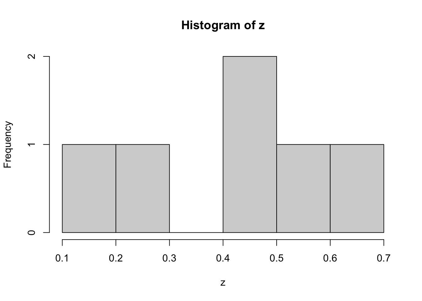
## [1] 1.667 1.667 0.000 3.333 1.667 1.667xts:

## [1] 1.667 1.667 0.000 3.333 1.667 1.667timeSeries:

## [1] 1.667 1.667 0.000 3.333 1.667 1.6672.2.9 能对金融时间序列对象应用 lag 函数吗?
lag 函数用以返回时间序列的滞后序列。
zoo:
## Z.1 Z.2 Z.3
## 2009-01-01 0.4770 0.5737 0.3990
## 2009-02-01 0.1829 0.5913 0.8642
## 2009-03-01 0.4473 0.9652 0.6136
## 2009-04-01 0.6603 0.5932 0.4981
## 2009-05-01 0.2228 0.2319 0.2083xts:
## X.1 X.2 X.3
## 2009-01-01 NA NA NA
## 2009-02-01 0.5087 0.5740 0.9311
## 2009-03-01 0.4770 0.5737 0.3990
## 2009-04-01 0.1829 0.5913 0.8642
## 2009-05-01 0.4473 0.9652 0.6136
## 2009-06-01 0.6603 0.5932 0.4981timeSeries:
## GMT
## S.1[1] S.2[1] S.3[1]
## 2009-01-01 NA NA NA
## 2009-02-01 0.5087 0.5740 0.9311
## 2009-03-01 0.4770 0.5737 0.3990
## 2009-04-01 0.1829 0.5913 0.8642
## 2009-05-01 0.4473 0.9652 0.6136
## 2009-06-01 0.6603 0.5932 0.49812.2.10 能对金融时间序列对象应用 lm 函数吗?
lm 函数用以拟合线性模型。可以用来进行回归、单层次方差分析和协方差分析(而 aov 函数提供了一个更方面途径来做这件事)。
zoo:
##
## Call:
## lm(formula = Z.1 ~ Z.2 + Z.3, data = Z)
##
## Coefficients:
## (Intercept) Z.2 Z.3
## 0.274 0.351 -0.110## 2009-01-01 2009-02-01 2009-03-01 2009-04-01
## 0.13534 0.04501 -0.20394 -0.09864
## 2009-05-01 2009-06-01
## 0.23236 -0.11014xts:
##
## Call:
## lm(formula = X.1 ~ X.2 + X.3, data = X)
##
## Coefficients:
## (Intercept) X.2 X.3
## 0.274 0.351 -0.110## 2009-01-01 2009-02-01 2009-03-01 2009-04-01
## 0.13534 0.04501 -0.20394 -0.09864
## 2009-05-01 2009-06-01
## 0.23236 -0.11014timeSeries:
##
## Call:
## lm(formula = S.1 ~ S.2 + S.3, data = S)
##
## Coefficients:
## (Intercept) S.2 S.3
## 0.274 0.351 -0.110## 2009-01-01 2009-02-01 2009-03-01 2009-04-01
## 0.13534 0.04501 -0.20394 -0.09864
## 2009-05-01 2009-06-01
## 0.23236 -0.110142.2.11 能对金融时间序列对象应用 lowess()函数吗?
lowess 函数的作用是基于局部加权多项式回归对对象进行 lowess 平滑。
zoo:
## $x
## [1] 1 2 3 4 5 6
##
## $y
## [1] 0.5336 0.4095 0.3747 0.4372 0.4124 0.2685xts:
## $x
## [1] 1 2 3 4 5 6
##
## $y
## [1] 0.5336 0.4095 0.3747 0.4372 0.4124 0.2685timeSeries:
## $x
## [1] 1 2 3 4 5 6
##
## $y
## [1] 0.5336 0.4095 0.3747 0.4372 0.4124 0.26852.2.12 能对金融时间序列对象应用 mad 函数吗?
mad 函数用以计算中位数绝对偏差,即上中位数和下中位数从中位数的偏离程度。
zoo:
## [1] 0.1814xts:
## [1] 0.1814timeSeries:
## [1] 0.18142.2.13 能对金融时间序列对象应用 median 函数吗?
median 函数的作用是返回简单中位数。
zoo:
## [1] 0.4622xts:
## [1] 0.4622timeSeries:
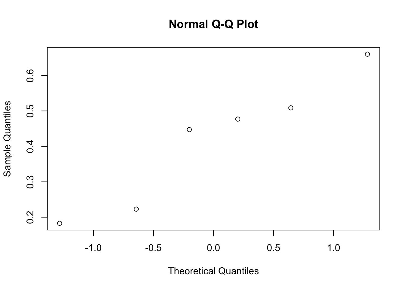
## [1] 0.46222.2.14 能对金融时间序列对象应用 qqnorm 函数吗?
qqnorm 函数用以绘制对象的 QQ 图;qqline 函数用以添加 QQ 线。
zoo:

## $x
## [1] 0.6433 0.2019 -1.2816 -0.2019 1.2816
## [6] -0.6433
##
## $y
## 2009-01-01 2009-02-01 2009-03-01 2009-04-01
## 0.5087 0.4770 0.1829 0.4473
## 2009-05-01 2009-06-01
## 0.6603 0.2228xts:
## $x
## [1] 0.6433 0.2019 -1.2816 -0.2019 1.2816
## [6] -0.6433
##
## $y
## X.1
## 2009-01-01 0.5087
## 2009-02-01 0.4770
## 2009-03-01 0.1829
## 2009-04-01 0.4473
## 2009-05-01 0.6603
## 2009-06-01 0.2228timeSeries:

## $x
## [1] 0.6433 0.2019 -1.2816 -0.2019 1.2816
## [6] -0.6433
##
## $y
## GMT
## S.1
## 2009-01-01 0.5087
## 2009-02-01 0.4770
## 2009-03-01 0.1829
## 2009-04-01 0.4473
## 2009-05-01 0.6603
## 2009-06-01 0.22282.2.15 能对金融时间序列对象应用 smooth 函数吗?
smooth 函数用以进行中位数平滑,该函数调用 Tukey 平滑器,如 3RS3R,3RSS,3R 等。
zoo:
## 3RS3R Tukey smoother resulting from smooth(x = z)
## used 1 iterations
## [1] 0.5087 0.4770 0.4473 0.4473 0.4473 0.4473xts:
## 3RS3R Tukey smoother resulting from smooth(x = x)
## used 1 iterations
## [1] 0.5087 0.4770 0.4473 0.4473 0.4473 0.4473timeSeries:
## 3RS3R Tukey smoother resulting from smooth(x = s)
## used 1 iterations
## [1] 0.5087 0.4770 0.4473 0.4473 0.4473 0.4473
2.3 金融时间序列对象与 utils 包中的函数
所需 R 包。
选取 utils 包中与金融时间序列对象分析相关的函数进行介绍。
常规数据
set.seed(1953)
data <-matrix(runif(18), ncol = 3)
charvec <-paste("2009-0", 1:6, "-01", sep = "")
charvec## [1] "2009-01-01" "2009-02-01" "2009-03-01"
## [4] "2009-04-01" "2009-05-01" "2009-06-01"zoo:
## Z.1 Z.2 Z.3
## 2009-01-01 0.5087 0.5740 0.9311
## 2009-02-01 0.4770 0.5737 0.3990
## 2009-03-01 0.1829 0.5913 0.8642
## 2009-04-01 0.4473 0.9652 0.6136
## 2009-05-01 0.6603 0.5932 0.4981
## 2009-06-01 0.2228 0.2319 0.2083xts:
##               X.1    X.2    X.3
## 2009-01-01 0.5087 0.5740 0.9311
## 2009-02-01 0.4770 0.5737 0.3990
## 2009-03-01 0.1829 0.5913 0.8642
## 2009-04-01 0.4473 0.9652 0.6136
## 2009-05-01 0.6603 0.5932 0.4981
## 2009-06-01 0.2228 0.2319 0.2083timeSeries:
## GMT
## S.1 S.2 S.3
## 2009-01-01 0.5087 0.5740 0.9311
## 2009-02-01 0.4770 0.5737 0.3990
## 2009-03-01 0.1829 0.5913 0.8642
## 2009-04-01 0.4473 0.9652 0.6136
## 2009-05-01 0.6603 0.5932 0.4981
## 2009-06-01 0.2228 0.2319 0.2083zoo:
## 2009-01-01 2009-02-01 2009-03-01 2009-04-01
## 0.5087 0.4770 0.1829 0.4473
## 2009-05-01 2009-06-01
## 0.6603 0.2228xts:
##               X.1
## 2009-01-01 0.5087
## 2009-02-01 0.4770
## 2009-03-01 0.1829
## 2009-04-01 0.4473
## 2009-05-01 0.6603
## 2009-06-01 0.2228
timeSeries:
## GMT
##               S.1
## 2009-01-01 0.5087
## 2009-02-01 0.4770
## 2009-03-01 0.1829
## 2009-04-01 0.4473
## 2009-05-01 0.6603
## 2009-06-01 0.22282.3.1 能对金融时间序列对象应用 head 函数吗?
函数用于返回 vector、matrix、table、data frame 对象的头部部分和尾部部分。
ts:
##  [1]  0.4736  0.4941 -0.3688  0.2365  0.6201
##  [6]  0.2098 -1.4904 -1.6032  0.6542 -0.1091
## [11] -0.6485 0.7964## [1] 0.4736 0.4941 -0.3688 0.2365 0.6201
## [6] 0.2098对于规则的 ts 类型时间序列,属性信息会丢失。
zoo:
##               Z.1    Z.2    Z.3
## 2009-01-01 0.5087 0.5740 0.9311
## 2009-02-01 0.4770 0.5737 0.3990
## 2009-03-01 0.1829 0.5913 0.8642## 2009-01-01 2009-02-01 2009-03-01
## 0.5087 0.4770 0.1829xts:
##               X.1    X.2    X.3
## 2009-01-01 0.5087 0.5740 0.9311
## 2009-02-01 0.4770 0.5737 0.3990
## 2009-03-01 0.1829 0.5913 0.8642## X.1
## 2009-01-01 0.5087
## 2009-02-01 0.4770
## 2009-03-01 0.1829timeSeries:
## GMT
##               S.1    S.2    S.3
## 2009-01-01 0.5087 0.5740 0.9311
## 2009-02-01 0.4770 0.5737 0.3990
## 2009-03-01 0.1829 0.5913 0.8642## GMT
## S.1
## 2009-01-01 0.5087
## 2009-02-01 0.4770
## 2009-03-01 0.1829